This article includes a list of general
references, but it lacks sufficient corresponding
inline citations. (March 2010) |
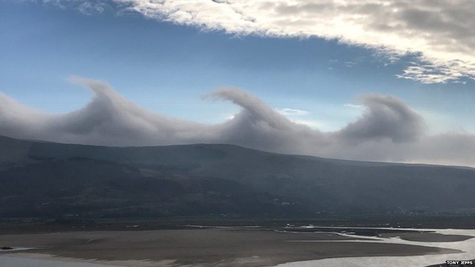
The Kelvin–Helmholtz instability (after Lord Kelvin and Hermann von Helmholtz) is a fluid instability that occurs when there is velocity shear in a single continuous fluid or a velocity difference across the interface between two fluids. Kelvin-Helmholtz instabilities are visible in the atmospheres of planets and moons, such as in cloud formations on Earth or the Red Spot on Jupiter, and the atmospheres of the Sun and other stars. [1]

Theory overview and mathematical concepts


Fluid dynamics predicts the onset of instability and transition to turbulent flow within fluids of different densities moving at different speeds. [3] If surface tension is ignored, two fluids in parallel motion with different velocities and densities yield an interface that is unstable to short-wavelength perturbations for all speeds. However, surface tension is able to stabilize the short wavelength instability up to a threshold velocity.
If the density and velocity vary continuously in space (with the lighter layers uppermost, so that the fluid is RT-stable), the dynamics of the Kelvin-Helmholtz instability is described by the Taylor–Goldstein equation:
![{\displaystyle (U-c)^{2}\left({d^{2}{\tilde {\phi }} \over dz^{2}}-k^{2}{\tilde {\phi }}\right)+\left[N^{2}-(U-c){d^{2}U \over dz^{2}}\right]{\tilde {\phi }}=0,}](https://wikimedia.org/api/rest_v1/media/math/render/svg/c6c95a25c4409c61a28f688c8f20f88f3ff49a5f)


Numerically, the Kelvin–Helmholtz instability is simulated in a temporal or a spatial approach. In the temporal approach, the flow is considered in a periodic (cyclic) box "moving" at mean speed (absolute instability). In the spatial approach, simulations mimic a lab experiment with natural inlet and outlet conditions (convective instability).

Discovery and history
The existence of the Kelvin-Helmholtz instability was first discovered by German physiologist and physicist Hermann von Helmholtz in 1868. Helmholtz identified that "every perfect geometrically sharp edge by which a fluid flows must tear it asunder and establish a surface of separation". [5] [3] Following that work, in 1871, collaborator William Thomson (later Lord Kelvin), developed a mathematical solution of linear instability whilst attempting to model the formation of ocean wind waves. [6]
Throughout the early 20th Century, the ideas of Kelvin-Helmholtz instabilities were applied to a range of stratified fluid applications. In the early 1920s, Lewis Fry Richardson developed the concept that such shear instability would only form where shear overcame static stability due to stratification, encapsulated in the Richardson Number.
Geophysical observations of the Kelvin-Helmholtz instability were made through the late 1960s/early 1970s, for clouds, [7] and later the ocean. [8]

See also
- Rayleigh–Taylor instability
- Richtmyer–Meshkov instability
- Mushroom cloud
- Plateau–Rayleigh instability
- Kármán vortex street
- Taylor–Couette flow
- Fluid mechanics
- Fluid dynamics
- Reynolds number
- Turbulence
Notes
- ^ a b Fox, Karen C. (30 December 2014). "NASA's Solar Dynamics Observatory Catches "Surfer" Waves on the Sun". NASA-The Sun-Earth Connection: Heliophysics. NASA.
- ^ Sutherland, Scott (March 23, 2017). "Cloud Atlas leaps into 21st century with 12 new cloud types". The Weather Network. Pelmorex Media. Retrieved 24 March 2017.
- ^ a b Drazin, P. G. (2003). Encyclopedia of Atmospheric Sciences. Elsevier Ltd. pp. 1068–1072. doi: 10.1016/B978-0-12-382225-3.00190-0.
- ^ Ofman, L.; Thompson, B. J. (2011-06-01). "SDO/AIA Observation of Kelvin-Helmholtz Instability in the Solar Corona". The Astrophysical Journal. 734: L11. arXiv: 1101.4249. doi: 10.1088/2041-8205/734/1/L11. ISSN 0004-637X.
- ^ Helmholtz (1 November 1868). "XLIII. On discontinuous movements of fluids". The London, Edinburgh, and Dublin Philosophical Magazine and Journal of Science. 36 (244): 337–346. doi: 10.1080/14786446808640073.
- ^ Matsuoka, Chihiro (2014-03-31). "Kelvin-Helmholtz Instability and Roll-up". Scholarpedia. 9 (3): 11821. doi: 10.4249/scholarpedia.11821. ISSN 1941-6016.
- ^ Ludlam, F. H. (October 1967). "Characteristics of billow clouds and their relation to clear-air turbulence". Quarterly Journal of the Royal Meteorological Society. 93 (398): 419–435. Bibcode: 1967QJRMS..93..419L. doi: 10.1002/qj.49709339803.
- ^ Woods, J. D. (18 June 1968). "Wave-induced shear instability in the summer thermocline". Journal of Fluid Mechanics. 32 (4): 791–800. Bibcode: 1968JFM....32..791W. doi: 10.1017/S0022112068001035. S2CID 67827521.
References
- Lord Kelvin (William Thomson) (1871). "Hydrokinetic solutions and observations". Philosophical Magazine. 42: 362–377.
- Hermann von Helmholtz (1868). "Über discontinuierliche Flüssigkeits-Bewegungen [On the discontinuous movements of fluids]". Monatsberichte der Königlichen Preussische Akademie der Wissenschaften zu Berlin. 23: 215–228.
- Article describing discovery of K-H waves in deep ocean: Broad, William J. (April 19, 2010). "In Deep Sea, Waves With a Familiar Curl". New York Times. Retrieved April 23, 2010.
External links
- Hwang, K.-J.; Goldstein; Kuznetsova; Wang; Viñas; Sibeck (2012). "The first in situ observation of Kelvin-Helmholtz waves at high-latitude magnetopause during strongly dawnward interplanetary magnetic field conditions". J. Geophys. Res. 117 (A08233): n/a. Bibcode: 2012JGRA..117.8233H. doi: 10.1029/2011JA017256. hdl: 2060/20140009615.
- Giant Tsunami-Shaped Clouds Roll Across Alabama Sky - Natalie Wolchover, Livescience via Yahoo.com
- Tsunami Cloud Hits Florida Coastline
- Vortex formation in free jet - YouTube video showing Kelvin Helmholtz waves on the edge of a free jet visualised in a scientific experiment.
- Wave clouds over Christchurch City
- Kelvin-Helmholtz clouds, in Barmouth, Gwynedd, on 18 February 2017
| Authority control databases: National |
|---|