
Size of this PNG preview of this SVG file:
720 × 540 pixels. Other resolutions:
320 × 240 pixels |
640 × 480 pixels |
1,024 × 768 pixels |
1,280 × 960 pixels |
2,560 × 1,920 pixels.
Original file (SVG file, nominally 720 × 540 pixels, file size: 19.82 MB)
| This is a file from the
Wikimedia Commons. Information from its
description page there is shown below. Commons is a freely licensed media file repository. You can help. |
Summary
| Description |
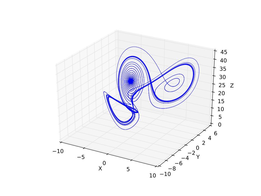
English: Modified Lorenz chaotic system by Miranda & Stone |
| Date | |
| Source | Own work |
| Author | Shiyu Ji |
Python Matplotlib Code
# A 3D Euler method based simulation of the Modified Lorenz System.
from mpl_toolkits.mplot3d import axes3d
import matplotlib.pyplot as pl
import numpy as np

t0 = 0.0
dt = 0.001
t_final = 100
T = np.arange(t0, t_final, dt)
a, b, c = 10.0, 8.0/3, 137.0/5
ax = pl.figure().add_subplot(111, projection='3d')
ax.set_xlabel('X')
ax.set_ylabel('Y')
ax.set_zlabel('Z')

x, y, z = -8.0, 4.0, 10.0
for t in T:
    f = 1.0/3/np.sqrt(x*x+y*y)
    dx = 1.0/3*(-(a+1)*x+a-c+z*y) + ((1-a)*(x*x-y*y) + (2*(a+c-z))*x*y)*f
    dy = 1.0/3*((c-a-z)*x-(a+1)*y) + (2*(a-1)*x*y + (a+c-z)*(x*x-y*y))*f
    dz = 0.5*(3*x*x*y - y*y*y) - b*z
    new_x = x + dx * dt
    new_y = y + dy * dt
    new_z = z + dz * dt
    ax.plot([x, new_x], y, new_y], z, new_z], 'b-', linewidth=0.5)
    x, y, z = new_x, new_y, new_z

pl.show()
Licensing
I, the copyright holder of this work, hereby publish it under the following license:
This file is licensed under the
Creative Commons
Attribution-Share Alike 4.0 International license.
- You are free:
- to share – to copy, distribute and transmit the work
- to remix – to adapt the work
- Under the following conditions:
- attribution – You must give appropriate credit, provide a link to the license, and indicate if changes were made. You may do so in any reasonable manner, but not in any way that suggests the licensor endorses you or your use.
- share alike – If you remix, transform, or build upon the material, you must distribute your contributions under the same or compatible license as the original.
File history
Click on a date/time to view the file as it appeared at that time.
| Date/Time | Thumbnail | Dimensions | User | Comment | |
|---|---|---|---|---|---|
| current | 09:20, 11 November 2016 |
| 720 × 540 (19.82 MB) | Shiyu Ji | User created page with UploadWizard |
File usage
The following pages on the English Wikipedia use this file (pages on other projects are not listed):